Delayed Mode Quality Control
Contents
8. Delayed Mode Quality Control
8.1. Correction for dynamic errors
Salinity derived from temperature and conductivity is prone to dynamic errors that are a result of profiling in a dynamic environment characterised by spatial temperature and salinity gradients. While dynamic errors in conductivity and temperature are usually small relative to natural variations, they can compound into large relative errors in derived salinity. This is because, in many regions of the ocean salinity does not vary as much as conductivity and temperature. Dynamic errors can, for example, create false density instability in profiles and false variation in mixed layer depths. This is particularly important in beta oceans, where density is set by salinity variations (e.g. in polar regions; Gulf of Oman). Both pumped, unpumped, electrode-based and inductive CTDs that measure conductivity and temperature (see Section 3), are prone to dynamic errors that can be greater than the instrument calibration accuracy and therefore need to be corrected for (Johnson et al., 2007), (Woo and Gourcuff, 2021).
Four main sources of error are (i) spatial offsets in sensor location on the profiling platform, (ii) timestamping of sensor measurements, (iii) the themister thermal-inertia effect and (iv) the conductivity cell thermal-inertia effect.
We suggest applying the thermal mass correction method similar to that proposed by (Garau et al., 2011), which was intially developed by (Lueck and Picklo, 1990) and (Morison et al., 1994), to account for the delayed temperature equilibration of the conductivity cell. (see Chapter 5 DMQC). The correction depends on the speed with which the water flows through the conductivity cell. For pumped CTDs, the flow through the CT cell is known and constant, thus corrections like (Garau et al., 2011) can be simplified to use only constant thermal-inertia corrections, however these corrections are generally worse around the thermocline because: 1) the glider speed may change as a result of stratification; 2) there is a rapid vertical change in temperature and/or salinity. In the case of unpumped CTDs, for increased accuracy, we recommend using the modelled velocity of the glider through the water (based on the flight model) to estimate the flushing speed of the CT cell, which can be used to correct for the temperature offset (reference to Depth Averages Current (DAC) SOP). The flight model can be improved by following pre-deployment and piloting protocols as per the DAC SOP. The amplitude of the error, ɑ, and the time offset constant, 𝜏, are used to correct for thermal mass offset. These parameters can be estimated by minimizing the difference between consecutive up and down dives in temperature and salinity space, although minimizing in salinity and depth space can be preferable in some environmental conditions (with different stratification characteristics) and was also applied by (Morison et al., 1994). We use up-down dives (the top of the yo) for this correction because the measurements are closest in time and space in the upper layer/thermocline where thermal-intertia errors tend to be most important. One can elect to apply this minimization per dive or over the whole mission. Per dive tends to give cleaner data but can sometimes mask real signals (if regressed in depth, z). Applying the minimization per mission makes the assumption that the shape of the sensor doesn’t change and that the model is representative and so only one set of parameters is needed to represent a whole mission. In cases in which the hydrodynamic coefficients change (e.g. if there is biofouling), per dive or multiple dive segments may be a preferable choice.
It should be noted that because such corrections require interpolating to a regular time grid, the (1) interpolation method and (2) correction scheme, can introduce energy at specific frequencies in post processing which can bias any form of spectral analysis for TS data down the line (https://oem.rbr-global.com/floats/files/5898249/34668603/1/1586804683000/0008228revA+Dynamic+corrections+for+the+RBRargo+CTD+2000dbar.pdf).
The corrections we propose are therefore:
8.1.1. Spatial alignment correction
Apply offset to account for the spatial offset in sensor location on the platform, if needed.
When the conductivity cell and thermistor are not colocated on the instrument, they measure the same water parcel but at different times. Similarly, the pressure sensor measurements for that water parcel will not occur at the same time. The time difference depends on the flow speed and distance between the sensors. If there is a variable profiling rate, the time difference will not be constant and the correction relies on the flight model. Pumped CTDs reduce the complexity of the correction by pumping water past the conductivity cell and thermistor at a known rate. The unpumped RBRlegato3 reduces the error associated with the sensor misalignment by moving the thermistor from the float end cap to the mast of the conductivity cell.
8.1.2. Interpolate to consistent timestamps
Interpolate to consistent timestamps between thermistor, conductivity cell and pressure sensors.
8.1.3. Correction for thermal inertia
Thermistors and conductivity cells have finite, but different, response times and are addressed separately.
8.1.3.1. Apply correction for thermistor thermal inertia
Heat must diffuse through a metal housing to reach the thermistor itself before a temperature change is registered. If a sensor has a long response time relative to the time scale for temperature changes, then the measured temperature will both lag the true signal, and have a reduced high-frequency amplitude. The error manifests itself as spikes in salinity and density especially when crossing interfaces with a sharp change in temperature with depth. The simplest correction it to shift temperature in time to ensure that the conductivity and temperature readings were taken simultaneously.
8.1.3.2. Apply correction for conductivity cell thermal inertia
Because conductivity is a function of both temperature and salinity, when the conductivity cell exchanges heat with the water it samples, errors can occur which manifest themselves as spikes in salinity or density when the instrument enters a mixed layer from stratified waters.
Initially, the effects of thermal inertia can be visualised as a scatter plot of temperature and salinity, colored by dive phase (whether the glider is performing a dive or a climb). The effectiveness of the correction can then be checked similarly. Often, the correction is not perfect: the remaining error can be reported as a RMSE of the difference between dives and climbs, as in (Giddy et al., 2021).
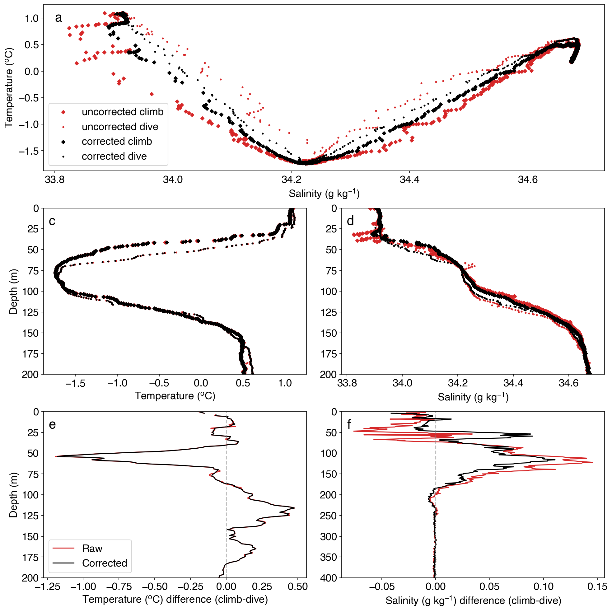
Fig. 8.1 Assessment of thermal inertia effects and its correction for one consecutive dive/climb sequence a) Uncorrected salinity and temperature; b) Corrected salinity and temperature; c) Uncorrected (red) and corrected (black) temperature-depth profile (both dive and climb); d) Uncorrected (red) and corrected (black) salinity-depth profile (both dive and climb); e) the temperature difference between a climb and a dive (uncorrected: red; corrected: black); f) the salinity difference between a climb and a dive (uncorrected: red; corrected: black). (Figure credit: Isabelle Giddy).
There are a number of implementations used by the community to correct for conductivity cell thermal inertia. These have generally been developed for specific sensor-platform integrations and are listed below as such.
8.1.3.2.1. Unpumped Seabird CT cell on seagliders
Basestation processing developed by Charlie Eriksen (unpublished). The correction is based on an iterative thermal diffusion scheme through layers in the water column.
8.1.3.2.2. Pumped Seabird CT cell mounted on Slocum gliders
GEOMAR implements the (Garau et al., 2011) method with updated coefficients.
8.1.3.2.3. Pumped and unpumped Seabird CT cell
8.1.3.2.4. SOCIB
SOCIB implements the (Garau et al., 2011) method.
8.1.3.2.5. UEA Glider Toolbox
UEA glider toolbox implements (Garau et al., 2011), using GEOMAR / Gerd Krahmann polynomials and an empirical regression of alpha and tau absolutes and offsets.
8.1.3.2.6. Integrated Marine Observing System (IMOS)
(Woo and Gourcuff, 2021) provide recommendations for the correction of thermal-inertia to both pumped and unpumped Seabird CT cells, following alignment of temperature measurements to the conductivity cell. In the case of pumped CTDs, the flow through the cell is constant and the method of (Lueck and Picklo, 1990), generalised by (Morison et al., 1994) is implemented. In the case of unpumped CTDs, the method developed by (Morison et al., 1994) is recommended over the more recent method by (Garau et al., 2011), which modified (Morison et al., 1994) to take into account variable flow speeds as a result of an unpumped CTD. Testing by (Woo and Gourcuff, 2021) found that the improvement in the correction algorithm did not improve the results and is computationally inefficient.
8.1.3.2.7. New method by Daniel Wang, Donglai Gong and Travis Miles (to be published)
An improved methodology is proposed by Daniel Wang, Donglai Gong and Travis Miles to correct the thermal lag error in pumped glider CTDs with a specific focus on glider data from the MAB and other highly stratified oceans. The method has been tested and validated on Slocum gliders with pumped Seabird CTDs. An updated thermal lag correction algorithm was developed based on (Garau et al., 2011) and it introduces a new cost function for calculating the pairwise thermal lag correction coefficients in highly stratified oceans. The algorithm also takes the vertical variability of the thermocline into account for more robust corrections in the presence of internal waves. Specifically, the parameters within the cost functions are normalized and depth is zero-referenced to the thermocline depth. Based on the observed temperature gradient at the thermocline, the algorithm then decides whether to use the normalized Temperature-Salinity or Salinity-Depth relation for the cost function. The improved method was able to eliminate most of the mismatches of salinity and density profiles between adjacent down up casts, and also fixed the problem of mismatching water mass identities in the Temperature-Salinity space. Salinity spikes up to 0.5 and density inversions up to 0.2 kg m-3 the vertical profiles were successfully corrected.
8.1.3.2.8. RBRlegato3
Recommended procedures by RBR themselves using internal and external temperature of the logger as detailed in their “Data processing and dynamic corrections for the RBRlegato3 CTD” report. Note that this work is still on-going, so the procedures are expected to be updated in the near future.
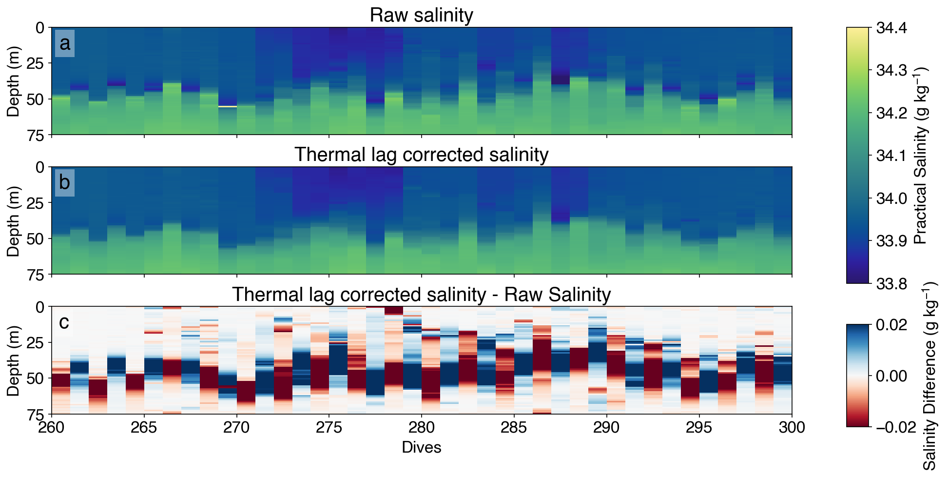
Fig. 8.2 Example of the thermal inertia effect on salinity before and after correction (Isabelle Giddy)
8.2. Sensor offset and drift correction
The sensor offset and drift are corrected using comparison CTD casts (see Section 5.1.1, Section 5.2.2). Temperature and salinity are regressed with a colocated CTD that has a known accuracy. Typically the salinity and temperature profiles are compared directly or in TS space. The sensor correction should be quoted together with details on the comparison cast. If no correction is made, this can also be reported.
8.3. Secondary cleaning and despiking
While thermal lag correction improves spikes and the dissymmetry between adjacent profiles, remaining outliers/spikes can be corrected for (depending on the use case) using rolling medians, depth-bins and the removal of outliers (e.g. some methods in GliderTools (Gregor et al., 2019)). The application of a median filter as proposed by (Liu et al., 2015) can further improve the salinity error correction in regions of strong thermoclines with temperature changes above ~2oC within 3 m.
8.4. Inter-comparison
To achieve long-term legacy datasets and help us understand inter-annual and inter-decadal variability, it is essential to ensure that the salinity observations are in-field delayed mode (DM) corrected to a world-class standard (Allen et al., 2020).
Significant effort from various manufacturers has been made to improve the CTD sensor’s stability and accuracy. Manufacturers will often quote a calibration capability of 0.002 oC and 0.0003 S m-1 for temperature and conductivity, respectively (see Section 3), however, calibrated instruments do not always meet this standard, particularly in salinity. In addition, 10-20 months of use, even at manufacturers stability figures, will double or even treble these differences, and to amplify this, two different vehicles may have instruments that have drifted apart in different directions. To achieve legacy value in historical observations, whether from gliders or any other observational platform, it is important that the typical magnitudes of large scale global change are resolvable by the quality of the historical data over a sensible time frame. NOAA’s Geophysical Fluid Dynamics Laboratory has a blog presenting global surface salinity trends, www.gfdl.noaa.gov/blog_held/14-surface-salinity-trends/, following (Durack and Wijffels, 2010) indicating that the largest long term global changes in salinity that can be expected even at the ocean surface is around 0.004 PSU per year.
Now that multi-platform observations are more and more common it is also important that inter-calibration procedures are routinely included between the data collected by different platforms. The ARGO profiling float community has been aware of the requirement for inter-calibration for some time (Owens and Wong, 2009) (Wong et al., 2003), and have valuable procedures in place to inter-calibrate float data as best they can. The huge growth in ocean observing data using glider vehicles provides a unique opportunity to support this initiative and take it further, particularly with the growing number of repeat monitoring lines that gliders have enabled and the resulting improvement in quasi-continuous observation of stable water masses and mode waters.
Cross calibration and validation of CTD profile data from any platform is not new (Bosse et al., 2015). For many decades, since the introduction of the electronic CTD, oceanographers have compared their CTD data, normally in θ (potential temperature)/salinity (θ/S) space, with historical profiles. This was to ensure that the short term stability of well studied, known stable water masses, and mixing lines, were not compromised by subtle instrument and/or laboratory anomalies. Salinity or temperature comparisons between datasets should always be made by plotting potential temperature against salinity on a θ/S diagram, as this is the best way to identify key characteristic water types in the vertical structure of the water; it overcomes the fact that both temporally and geographically, characteristic water types can be found at significantly different depths in the water column, which can vary significantly on short timescales due to processes such as Internal Waves and the propagation of eddies.
For gliders, a semi automatic inter-calibration correction pack has been developed by SOCIB to field correct its glider data (Allen et al., 2020), both for regular monitoring lines and for specific process study programmes: it is available through GitHub at https://github.com/socib/salinity-correction-toolbox, and explained in the manual found at repository.socib.es/repository/entry/show?entryid=74d6c56a-0c87-4790-8e0b-5896b540557c. The contribution to Ocean Best Practices is provided at repository.oceanbestpractices.org/handle/11329/884. For SOCIB monitoring lines such as that across the Ibiza and Mallorca channels this is generally quite straightforward as short (3 day) seasonal research vessel cruises are carried out to enable a laboratory analysis constraint for the quality of the semi-continuous glider monitoring. More disparate glider missions for process studies, require more manual intervention in the selection of well calibrated CTD reference data. In both cases however, particular turning points (water types), and mixing lines (water masses), in the θ/S diagrams, are compared to identify the difference between the uncorrected glider data and the water bottle corrected ship CTD data.
We appreciate that some facilities, laboratories and operators may not have access to their own reference bottle calibrated lowered CTD data sets. In this case, local, national or international databases may need to be relied upon. Good databases will have levels of confidence or accuracy to the quality of the calibrated data provided in their metadata. Ideally the vertical resolution of the reference datasets should be approximately the same as or better than the glider data, i.e. ~ 1 m or 1 db, or better. Again, most good databases should be able to supply this. Lower vertical resolution will have some limiting effect on the quality of the final result, although interpolation of the data may afford an acceptable cross-calibration.
Shallow glider data and shallow water applications for glider platforms may be unsuitable for delayed mode inter-calibration as presented in this paper. Stable and well defined water masses and mixing lines are not common in near surface or shallow waters, where high frequency air-sea interaction processes can effect water temperature changes and freshwater input independently and lead to considerable variability in θ/S space. For these applications, the operator may not be able to do better than to accept the error in manufacturer’s instrument calibration and instrument drift, unless they have access to their own calibration facilities or a mechanism for taking bottle samples very close to the glider vehicle.
Sensor drift corrections to shipboard CTD casts and/or other gliders should be reported (see GROOM-FP7 D5.3).