Delayed Mode Quality Control
Contents
8. Delayed Mode Quality Control
8.1. Calculation of oxygen variables
Following (Bittig et al., 2018).
8.2. Sensor drift correction
Aanderaa describe the in-situ drift characteristics of the 4330 and 4831 series optodes as being < 0.5 % per year, and they make no distinction between the standard or fast (“F”-type) foils (Tengberg and Hovdenes, 2014). Optodes made after 2016 undergo a “burning-in period” during manufacture and therefore have substantially less drift (Tengberg and Hovdenes, 2014). Drift is a function of UV exposure and sampling frequency. The foil becomes less sensitive and therefore drift is always towards lower oxygen concentrations. The drift is believed to be due to bleaching of the luminophore foil via ambient light; it is particularly sensitive to fluorescent lights. The bleaching effect is partly counteracted by a destabilizing effect on the luminophore. Together this manifests as a positive factor on the oxygen concentration (slope > 1) and a positive offset at zero oxygen.
(Queste et al., 2018) recorded drifts of 0.0176 and 0.0109 μmol kg-1 day-1 for two Seagliders using inflections in the oxygen profiles as the glider penetrated to Arabian Sea Oxygen Minimum Zone and the sodium sulphite method, but no Winklers. (Bittig and Körtzinger, 2015) report a 10 % drift over 3 years, but this is a combination of in-situ and ex-situ drift. (Bittig et al., 2018) determined the drift to be typically 0.1-0.2 % per year in-situ. A drift of 0.0004 % day-1 has been calculated based on UEA seagliders against Baltic deep water oxygen climatology (Possenti et al., 2021). Values between 0.0004 and 0.0035 % d-1 have been found across 16 vehicles in-situ: slocums and seagliders with 4330F (old foil formulation), 4835 and 4831 optodes (Tom Hull personal communication).
The drift correction should be applied to the oxygen concentration, not the measured phase (Bittig et al., 2018).
8.3. Sensor time response correction
In all but more important in the most homogeneous waters it is essential to correct for the slow time response of optodes (Bittig et al., 2014), (Bittig and Koertzinger, 2017) (see Fig. 8.1). This is particularly critical for optodes using the “standard” black foils, and as previously mentioned Slocum gliders with the optode in the standard location near the tail of the glider (Moat et al., 2016).
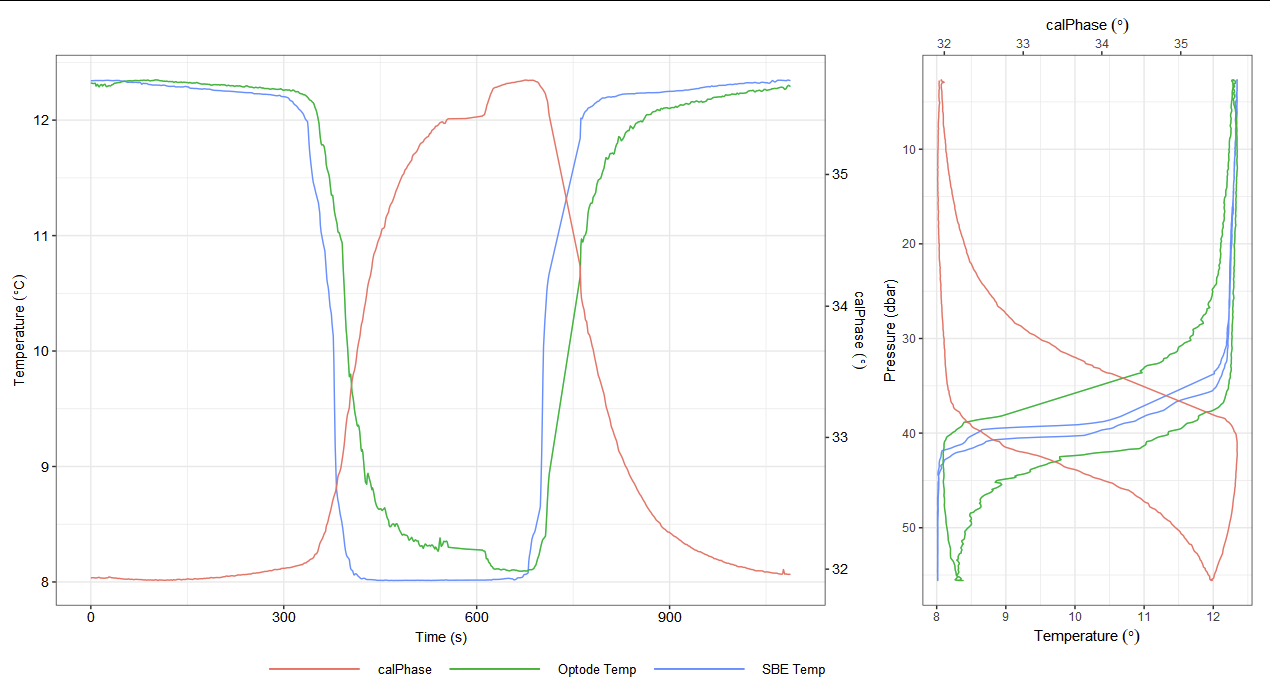
Fig. 8.1 Example uncorrected profiles from AlterEco AE5 “Kelvin” Slocum with a 4831 optode with standard foil demonstrating significant lag in both optode temperature and phase.
Correction requires the collection of optode phase, temperature and time. Therefore, the instruments and gliders should be configured to collect these variables and not just oxygen concentration or saturation. If only optode temperature and concentration are recorded, routines exist to recalculate phase, but this can introduce some inaccuracy and best to avoid it. Accurate time-stamps for these data are required to be able to perform this correction. Many data processing routines may remove these timestamps, such as to place the oxygen data on the same time-axis as the CTD, but for best results the oxygen sensor time should be used for the time response correction before interpolating to match the CTD. Users should be aware that many gliders have independent guidance-control computers and sensor computers and timestamps may differ between them. An important note is which temperature, be it optode or CTD, is used for the correction. The optode temperature typically has a lower accuracy and a slower response.
The lag is caused by a combination of factors, the relevance of these changes depending on the environment, optode type and glider platform. The rate of diffusion across the membrane (foil) is controlled by the water temperature and the thickness of the foil. Diffusion across the boundary layer above the membrane is also temperature dependent, but also influenced by the flow of water, which is determined by the position of the sensor and the glider speed and/or angle of attack. Lastly geometric lag is caused by a delay in water reaching the sensor due to glider geometry and the flow path of the surrounding water.
The boundary layer diffusion lag and the geometric lag will also affect the optode temperature response, which itself may have a time response due to the type of PRT used. As noted above, the type 3835 optodes have particularly slow responding temperature sensors. It is typical for users to use the CTD temperature in these instances.
The ideal correction method is still a point of discussion. We suggest users try each of these procedures and assess how well they work for their own use case.
8.3.1. Time response correction 1 - GEOMAR
Optode calibration and processing methods were developed by Johannes Hahn in collaboration with Henry Bittig for use on moored and glider-attached Aanderaa optodes. A set of routines were adapted to the particularities of optodes on gliders and to the typical conditions of GEOMAR glider deployments. This processing has now been used on nearly 100 glider deployments mostly in the Tropical Atlantic and Pacific Oceans (Krahmann et al., 2021). The processing determines two delay time constants. One \(\tau_{CTD}\) describes the time constant of an exponential filter which, when applied to the glider’s CTD temperature, gives an estimate of the temperature of the optode foil. And the other describes the optode response time to changing oxygen concentrations. The processing so far makes no explicit correction for the “geometric” lag, that is any lag introduced by the CTD and optode being some distance from each other. This “geometric” lag should be of the order of a few seconds and thus is significantly smaller than the other two delay time constants. Implementing and correcting such a lag should however be fairly simple.
To determine the two time constants a number of steps are performed:
Linearly interpolate optode phase, optode temp, CTD temp, pressure and salinity variables onto 1 sec grid to avoid issues from different measurement times.
A set of foil temperatures is estimated by applying an exponential filter to the CTD temperature with time scales from 10 to 50 s (in steps of 5 s), thereby creating different ‘virtual’ foil temperatures.
With this set of virtual foil temperatures, oxygen concentrations are calculated using either the Aanderaa supplied or the own-calibration derived set of optode coefficients.
For each of the resulting oxygen concentrations a reverse exponential filter with time scales of 0 to 200 s (in steps of 20 s) is applied to create sets of oxygen concentration profiles.
These sets of concentration profiles are then filtered with a forward-backward filter (MATLAB
filtfilt) to remove the noise introduced by the reverse filtering. Currently, a fixed time constant of 40 s is used for this filter. Depending on whether fast or slow foils are used, other values might deliver better results.All concentrations are gridded to a 1 dbar grid (first binned and then linearly interpolated to the full dbar).
Differences between all up-down pairs are calculated and summed up for each of the concentration sets.
The one delay pair (CTD-temp delay for virtual foil temperature & Optode response delay) with the smallest difference sum is chosen and applied to the whole deployment.
Typically, the ‘best’ delays are CTD-temp: 30-100 s, optode response : 20-50 s.
Include into the optimization only up-down pairs that were not influenced by obvious bio-fouling.
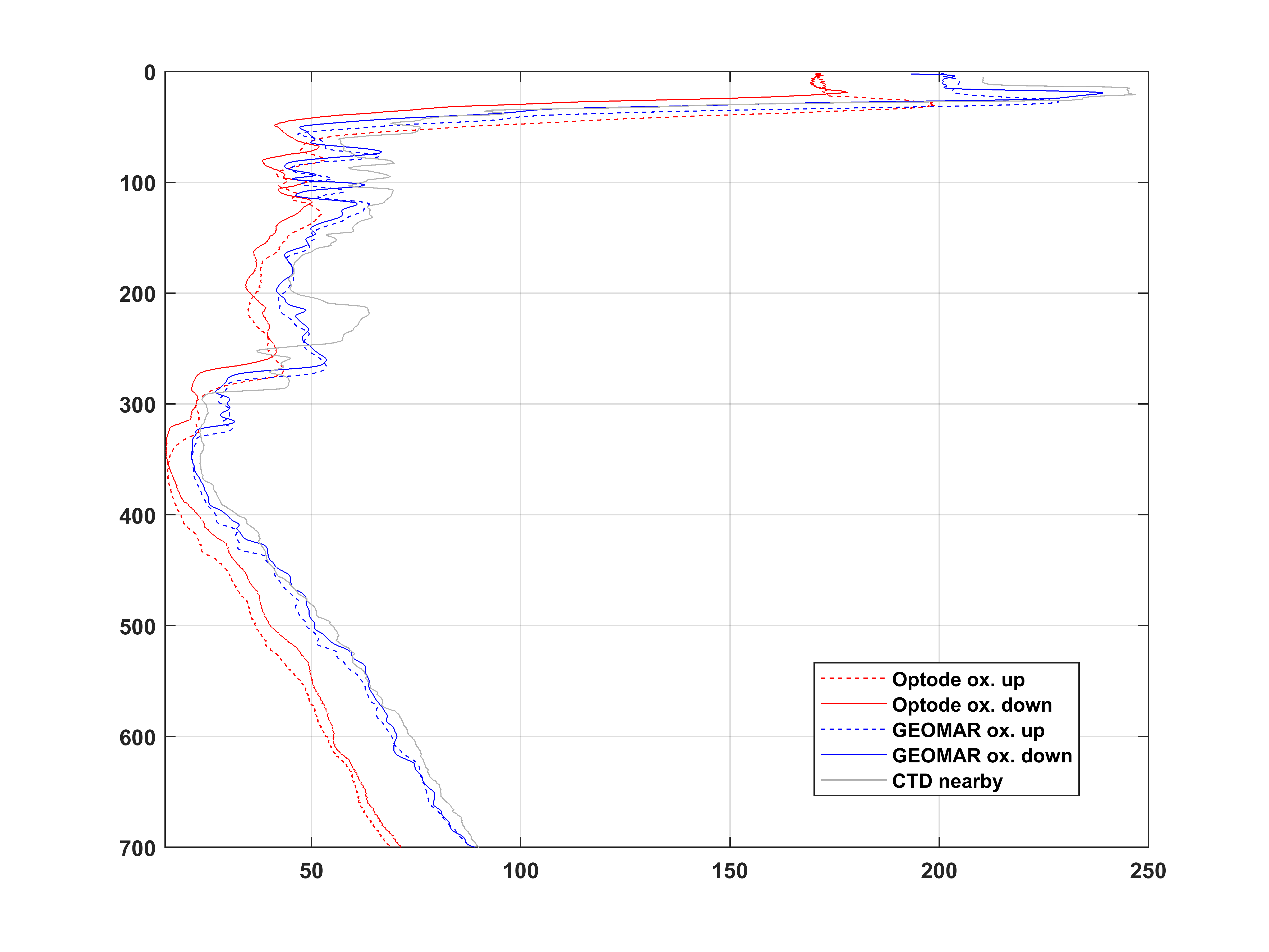
Fig. 8.2 Example of original Optode oxygen concentrations (red) and GEOMAR processed and calibrated (blue) oxygen concentrations. Shown is an up-down pair from a deployment off Angola. Solid lines are the up and dashed lines the down data. Also shown are calibrated oxygen concentrations from a nearby and contemporaneous CTD cast.
8.3.2. Time response correction 2 - IMOS
The routine developed by Mun Woo for the IMOS (Slocum) glider toolbox compares up and down casts in pressure space, but applies a time-shift rather than an exponential filter (Woo and Gourcuff, 2021). These time-shift values are determined per dive, but a rolling median is calculated to exclude dives with very high or low lag values.
The advantage of this method is that it does not amplify noise which the filter will tend to do. However, simply shifting the optode data relative to time will not remove some second order effects.
A \(\tau\) for the geometric component of the lag is determined from the average pitch and average vertical speed for each cast.
These values are filtered to avoid extreme values.
A linear time shift using the filtered \(\tau\) is then applied to align the optode phase and CTD parameters (typically 4 seconds).
Then, for the diffusive lag, the median RMS difference and bias between up and down cast is calculated over a range of possible \(\tau\) values (0 to 40 seconds) for each dive.
A time shift is then applied to the optode phase with the \(\tau\) which minimized the median RMS difference.
Oxygen concentration is then calculated using the corrected phase and CTD temperature following using the factory foil coefficients.
8.3.3. Time response correction 3 - UEA
The routine developed by Bastien Queste for the UEA Seaglider toolbox works as follows:
The CTD temperature is aligned based on flight speed to the optode phase using a 1-D interpolation and a flight speed dependent time-shift. (the optode and Sea-Bird temperature are close together on a Seaglider so the time-shift is small).
Oxygen partial pressure is calculated using the optode phase and time shifted optode temperature.
Up and down profiles are compared (in pressure or density space depending on environmental conditions) and either:
A shoelace algorithm is used to minimize the area between the curves or
The RMSD from vertically binned data is calculated
A minimization algorithm (
fminsearchfrom MATLAB) is used to fit two lag coefficients: \(\tau = \tau_0 + \tau_1 (T-20)\) as per @Hahn2014.This \(\tau\) is then used with an exponential inverse-filter, typically against optode phase (and oxygen recalculated) but partial pressure or concentration as per (Bittig et al., 2018) has also been tested. The correction is applied on a per-dive basis.
Oxygen concentration is then calculated using the corrected phase and CTD temperature following using the factory foil coefficients.
8.3.4. Time response correction 4 - AlterEco
For AlterEco, many gliders were not collecting data on both up and down casts which precludes the use of the above routines. The routine implemented by Tom Hull was as follows:
A \(\tau\) was calculated for the geometric and boundary layer diffusive lag by minimizing the difference between the CTD and optode temperatures.
This \(\tau\) was used to then inverse-filter the optode phase and temperature.
A secondary lag correction based on the temperature as per the UEA toolbox and (Hahn et al., 2014).
Oxygen concentration is then calculated using the corrected phase and optode temperature following using the factory foil coefficients.
8.4. Light intrusion
Optodes can be sensitive to light intrusion if the foil is damaged. These instruments will typically still provide good data in the absence of light. A check should be made for increased sensor noise near the surface during daylight hours and contrast this with nighttime observations.